Machine learning applications span many business domains. One of the industries that I have a keen interest in is the stock market. I always wondered how the prices moved and what moved them.

I was so involved in this research that I wrote a book about it. You can find it here on Amazon if you wanna know how prices moved and how you can benefit from it.

While I'm learning data science and machine learning, I saw many predictive models that can read and learn relationships between several data points and somehow provide a future prediction. Examples include weather forecasts, sales predictions, game scores etc.

So naturally, as an avid stock market enthusiast, I wanted to put my machine learning skills to check if I can build a model that can predict any stock's future price.

This blog showcases the technique I used to train a model that can spit out the next day's closing price of any stock symbol.

Are you ready?

Here's the Kaggle notebook for you to check out.

Understanding stock prices

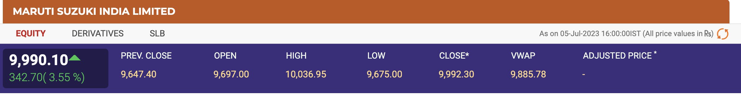
In the pic above, you can see the performance of the day for a stock Maruti Suzuki India Limited (symbol: MARUTI).

Among the numbers you see, we are interested in the following:

• OPEN - this is the price at which the market opened today for this stock

• HIGH - this is the lowest price point for this stock during the day

• LOW - this is the lowest price point for this stock during the day

• CLOSE - this is where the price finally landed at the end of the market's closing

this is a stock from the NSE (National Stock Exchange) of India but the same metrics can be observed for any stock on any exchange in the world.

We can see the same open, high, low, and close prices for any stock symbol.

The 'close' price is what we are most interested in because that is what we are going to predict. This is the number that tells us where the stock price is going to finish the next day.

The model we are going to build should tell us the closing price of a stock for the next day.

For any model building, we are going to need training data. The model learns from this training data which we can then apply on test data to see how well it is performing.

Let's see how we can get this training data.

Building a training data set

There is a Python library maintained by Yahoo that provides real-time stock prices for any stock. The library is called "yfinance" and we are going to use that to build our training data set.

From this library, we can get many metrics about any stock such as dividends, capital gains, balance sheets, cash flow statements etc and we don't need all that for now.

We are going to use just one function from the library which can give us the history of any stock's price behaviour.

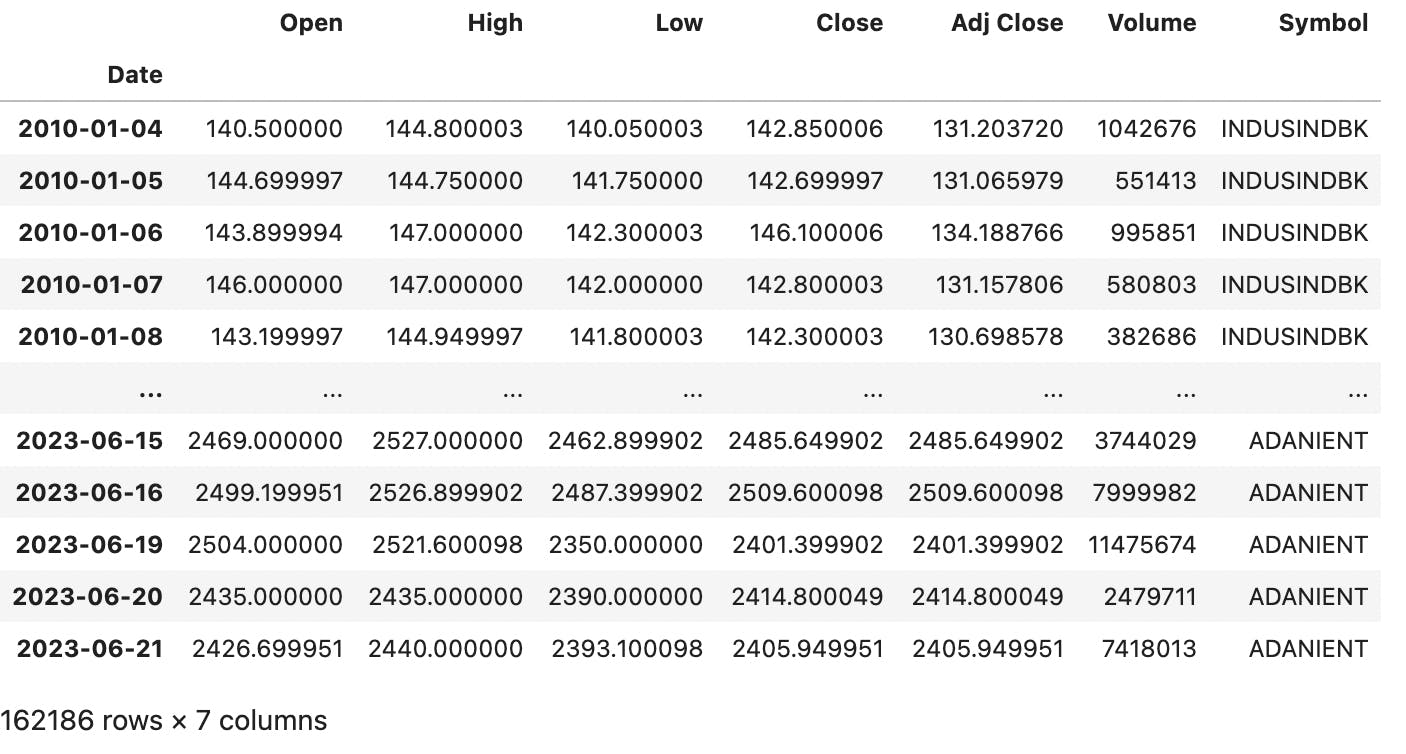
yf.download('INDUSINDBK', start="2010-01-01", end="2023-06-22")

which will give us data such as below.

As we discussed in the previous section, we are going to use the open, high, low, and close data points to build a model that can predict the future close price of a stock.

Ok, enough theory, let's get into coding.

Data preprocessing

First, install the necessary libraries.

import pandas as pd
import numpy as np
import matplotlib.pyplot as plt
import yfinance as yf
import tensorflow as tf
from sklearn.preprocessing import StandardScaler,MinMaxScaler
from sklearn.model_selection import train_test_split
from tensorflow.keras.models import Sequential
from tensorflow.keras.layers import LSTM, Dense

You can see that we are going to use the base utilities like pandas, numpy and matplotlib, then the yfinance to get our price data, and then we have the libraries required for model building from tensorflow and sklearn. We'll talk about them in a bit.

By the way, if you are working on Kaggle and don't know how to install external libraries like 'yfinance', you can check the instructions for it in my other post here.

Adding external libraries to Kaggle Notebook

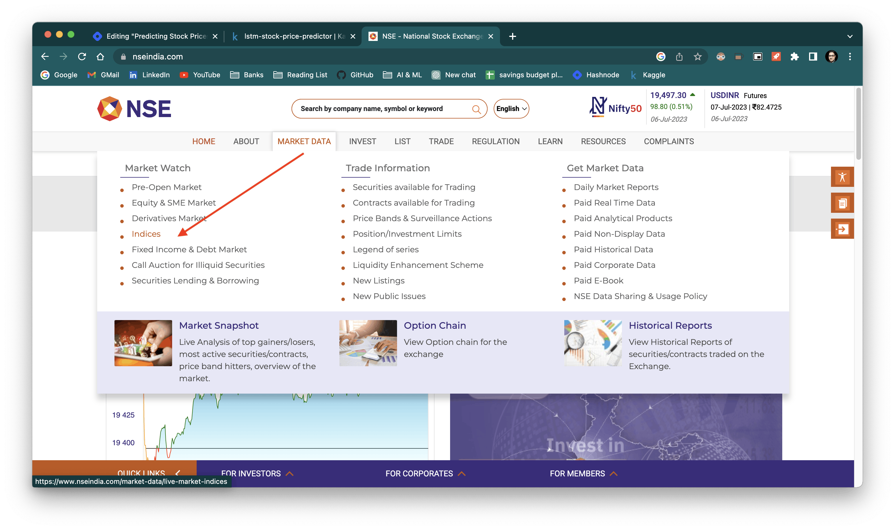
To get the training data, I went to NSE India's website and downloaded the list of stocks under the NIFTY 50 index. You can do the same by following the screenshots below.

Add the CSV file to Kaggle's input folder using the upload icon.

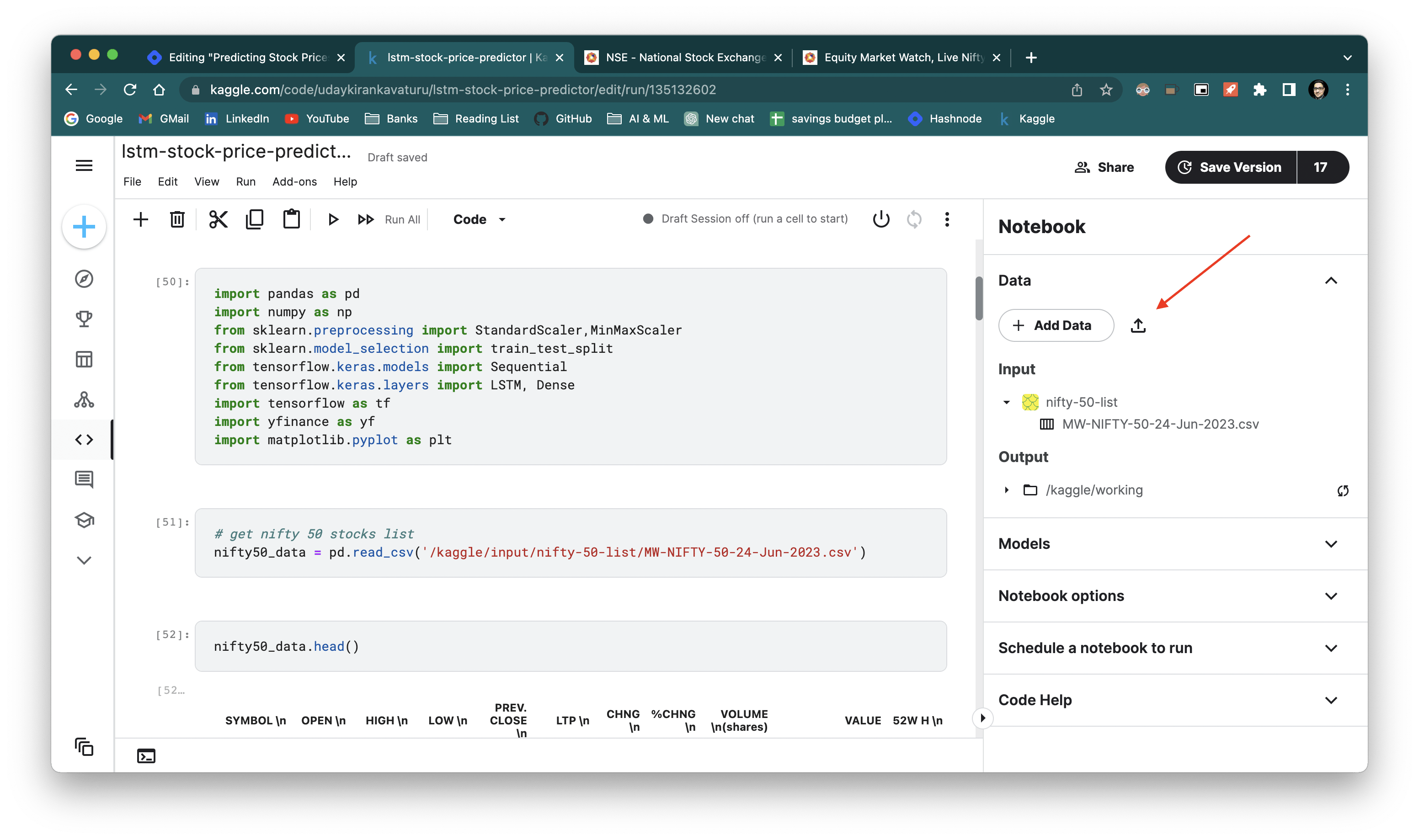
Once we have the file let's read the data from the CSV file using pandas.

# get nifty 50 stocks list
nifty50_data = pd.read_csv('/kaggle/input/nifty-50-list/MW-NIFTY-50-24-Jun-2023.csv')

There are many data fields in the CSV, we are interested in only the stock symbols in this NIFTY 50 index. Let's extract them.

# Extract the stock symbols
nifty50_stocks = nifty50_data['SYMBOL \n'].tolist()

print(nifty50_stocks)

Output:

For each of the 50 stocks, let's download the stock price history for a long date range. We can use 'yfinance''s download function to get the price data.

dfs=[]
for stock in nifty50_stocks:
    stock_data = yf.download(f'{stock}.NS', start="2010-01-01", end="2023-06-22")
    stock_data['Symbol'] = stock
    dfs.append(stock_data)
data = pd.concat(dfs,axis=0)

This is what the extracted data looks like so far.

Next,

data_list = []
scaler = MinMaxScaler(feature_range=(0,1))
for index,symbol in enumerate(symbols):
    symbol_data = data[data['Symbol']==symbol][['Open','High','Low','Close']]
    if symbol_data.shape[0] == 3325:
        scaled_data = scaler.fit_transform(symbol_data)
        data_list.append(scaled_data)

The above code is an important pre-processing step. Let's go through it in detail.

First, we created a scaler object using the MinMaxScaler from Scikit learn library. We need this to convert each price point to a standard scale.

We do this in any model-building pre-processing exercise to ensure that there are no major outliers that skew the training process which can lead to false learning.

We have provided a range (0,1) to the MinMaxScaler which means that the object will convert any numeric data point within the range of 0-1.

Then, we go through each stock symbol, extract the Open, High, Low, and Close data points from the downloaded data and ignore the rest.

Then, we scale each extracted data point using the scaler object resulting in a value between 0,1.

Then, finally, we add all these data points to a list.

Note: we used the if condition "if symbol_data.shape[0] == 3325" for consistency. Not all stocks have the price information for all dates in the given date range. So after the above code block is done, we have a 3-dimensional NumPy array of shape (46, 3325, 4).

This means that we have 3325 rows for each of the 46 stocks with 4 columns in each row (open, high, low, close).

We now have the data in the shape we want. Let's move on to the model building.

We are going to build an LSTM model. Let's quickly understand what LSTM is.

LSTM is a variant of RNNs which is a type of deep learning ANN network. If you don't know what any of these mean, here's a brief background without any of the math.

What is deep learning?

Deep learning is a field of science that makes the computer mimic the human brain.

pic credit: bdtechtalks.com

In the human brain, there are millions of neurons. Each neuron processes data individually and they 'spark' meaning that it either activates or it doesn't. Collectively, a group of neurons send their activation status which forms some context. This context is then passed on to the next group of neurons which produces its output to provide even more context.

There are many groups like this in our brains which are working in tandem to make us interpret the outside world.

pic credit: mathworks.com

When we see a dog with our eyes, the brain's neurons process each viewpoint(pixels) and collectively decide that it is a dog. And then the body reacts to it.

pic credit: datacamp.com

So when you want to bring this capability of the brain to the machine, we employ some techniques from the field of science called deep learning.

It's called deep because of the dense layers that go deep as needed to make the machine correctly perform its task such as object detection.

These layers provide the computer with the ability to learn collectively using something called neurons and collectively the neurons form a group called layers and the layers form a network. We refer to this network as Artificial Neural Network (ANN).

We can design and train such networks for any particular task such as the classification of images, finding defects in X-rays, predicting company sales etc. Any regression and classification problem can also be solved through these artificial networks. But since these are deep networks, they are compute-intensive. So a trade-off needs to be made when making a model selection.

In a task where we are building a model to predict a company's sales, we might be using a dataset in two dimensions i.e., there are many rows of the company's past sales over the years with many columns such as customer data, order history etc.

We can build an ANN around this type of dataset and make a predictive model. But when it comes to dealing with images simple ANNs can't be used because there is a third dimension involved.

Each image is typically an array of pixels of height and width but there is also a third property called the color channel (RGB).

pic credit: oreilly.com

So when a new dimension is introduced to our dataset, we also need to adapt and use a different type of ANN to deal with datasets with images.

Those are called Convolutional Neural Networks.

Convolutional Neural Networks

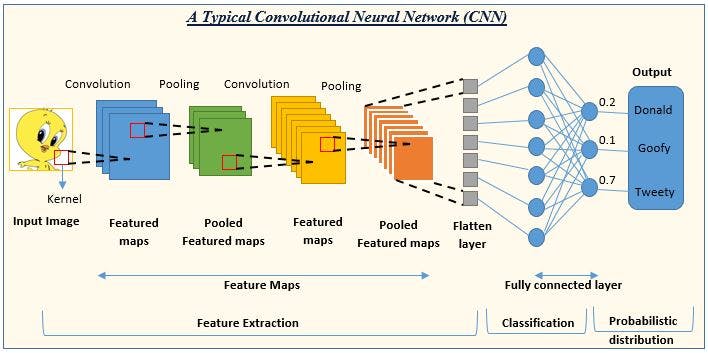
pic credit: analyticsvidhya.com

Let's not get too bogged down with the details of the above CNN architecture. The only takeaway here is that when a 3-dimensional data set such as images is given to us, CNNs can be used to extract details from the image and train themselves on any task such as the classification of images.

In the above example, a picture of Tweety is given and a dense CNN layer is trying to identify it as Tweety.

Now let's take it a step further.

Let's say we have videos to analyse. Now videos are nothing but a set of images put together in a sequence.

In a video dataset, each data point is no longer a 2-D or 3-D but now it's 4D. Because each data point is a video, each video is a sequence of images and each image is a sequence of pixels with RGB channel. Each image inside a video is also sequential in nature i.e., the second image only makes sense when it comes after the first image, the third image only makes sense when it comes after the second image and so on.

To deal with such a dataset we no longer can use CNNs, but we need to go to the next type of ANN called the Recurrent Neural Network which can deal with a higher dimension.

Recurrent Neural Network

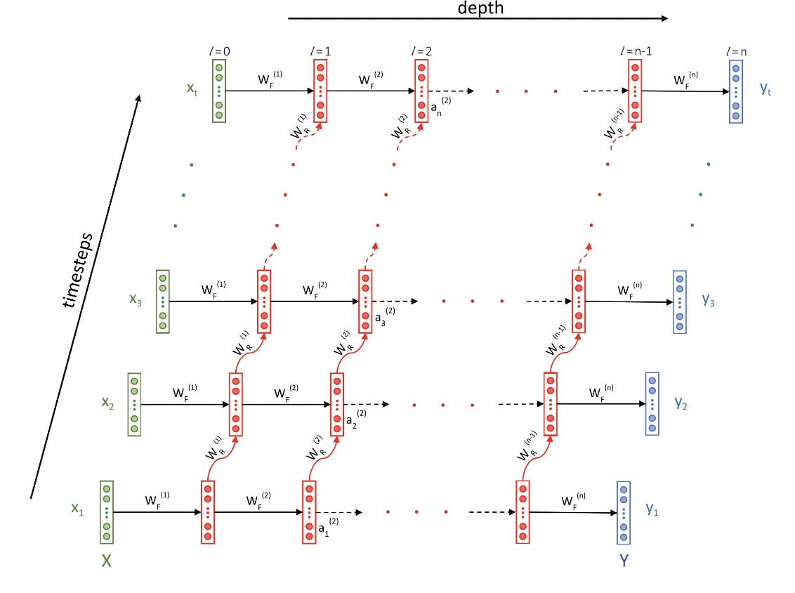
pic credit: upgrad

In the picture above, you can see the depth of the network in the x-axis which is typically the same as any ANN, but now there is a new y-axis which takes care of sequence in each data set.

So here, when a video with an image sequence is provided to the network, it is not only going through each image independently, but it is also learning the relationship with previous images in the video as a whole.

In a video classification problem such as gesture recognition, each video is analysed to check if a gesture is present or not. If present, the type of gesture needs to be identified. So each image (frame) within a video is checked for patterns using an image sequence.

Now, coming back to our stock price prediction problem, we have 46 stocks, and each stock has a time series of open, high, low, and close price points. Each price point is dependent on the previous date's price point because it then shows the journey of the stock's price across dates. This makes it a perfect candidate for using an RNN because it can learn each stock's behaviour using past performance which is exactly what we need it to do.

But wait, didn't I say LSTM?

Yes, let's get to that now.

LSTM is just a variant of an RNN and it was created to solve a fundamental problem with the RNN network called the exploding and vanishing gradients.

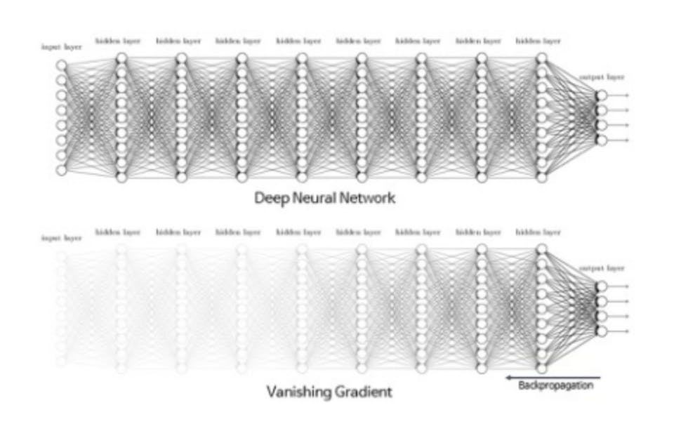
pic credit: Kaggle

To understand this problem, we'll need a full understanding of the inner workings of the RNN which is not the purpose of this blog. If you're curious, please check this website to understand it better.

For now, please trust me when I say this. LSTM is a type of RNN which is better than a regular RNN.

LSTM stands for Long Short Term Memory, and because it has an inner memory feature it solves the above-mentioned problem with a typical RNN.

So our LSTM model is going to look at patterns within the time series of each stock. It's going to look at these patterns for each of the 46 stocks we are going to give it and learn common patterns among all the stocks. When it's ready we can use that model to predict the next day's prices.

Are you with me so far? Good.

Let's get to the model building which is actually the easiest part once you know the above theories.

Model building

We now have a dataset of (46, 3325, 4). Let's split these into train and test data. Let's also extract the last record so we can use it as a target variable.

# Split the data into train and test sets
train_data, test_data = train_test_split(data_array, test_size=0.2)

# Prepare the input and output data for the LSTM model
train_input = train_data[:, :-1, :]  # Use all but the last time step as input
train_output = train_data[:, -1, :]  # Use the last time step as output

test_input = test_data[:, :-1, :]
test_output = test_data[:, -1, :]

Here we have used sklearn's test_train_split function. We provided a test_size of 0.2 which is 20% of the full data set. 80% will be used for training, 20% for testing and evaluation of the model.

# Build the LSTM model
model = Sequential()
model.add(LSTM(64, input_shape=(train_input.shape[1], train_input.shape[2])))
model.add(Dense(4))  # Assuming you want to predict 4 values
model.compile(loss='mean_squared_error', optimizer='adam')

The above code is how we define the LSTM model.

In the first layer, we are using 64 kernels to train the input data. Next is the Dense layer which will provide the final output record.

For model compiling we are using the standard 'mean_squared_error' as the loss function along with the 'adam' optimizer.

If you wanna know about these loss functions and optimizers, please check this website.

Now let's fit the model on the training data.

# Train the model
model.fit(train_input, train_output, epochs=10, batch_size=32)

I have used 10 epochs with a batch_size of 32, please feel free to experiment further.

Let's see how the model is performing.

Model evaluation

There are a couple of ways I evaluated the model. One is of course the standard loss check on the test data.

# Evaluate the model
loss = model.evaluate(test_input, test_output)
print("Test loss:", loss)

Output: Test loss: 0.024268725886940956
This is pretty neat I would say.

From here I reverse-engineered to check if the predicted prices are close enough to the actual prices.

# Get the models predicted price values 
predictions = model.predict(test_input)
predictions = scaler.inverse_transform(predictions)

# extract last time step closing prices
test_input_closing_prices = []
for data in test_input:
    inverse_data = scaler.inverse_transform(data)
    test_input_closing_prices.append(inverse_data[-1][-1])

test_output_closing_prices = []
inverse_data = scaler.inverse_transform(test_output)
for data in inverse_data:
    test_output_closing_prices.append(data[-1])

And then plot a graph to check the differences

# Compute the difference between the values in the two lists
difference = [abs(a - b) for a, b in zip(test_input_closing_prices, test_output_closing_prices)]

# Create the plot
plt.plot(test_input_closing_prices, label='Actual Closing Prices')
plt.plot(test_output_closing_prices, label='Predicted Closing Prices')
# plt.plot(difference, label='Difference')

# # Display values on the graph
# for i, val in enumerate(test_input_closing_prices):
#     plt.text(i, val, str(val), ha='center', va='top')

# for i, val in enumerate(test_output_closing_prices):
#     plt.text(i, val, str(val), ha='center', va='bottom')

plt.xlabel('Index')
plt.ylabel('Value')
plt.title('Actual vs Predicted Values in Test Set')
plt.grid(True)
plt.legend()

# Show the plot
plt.show()

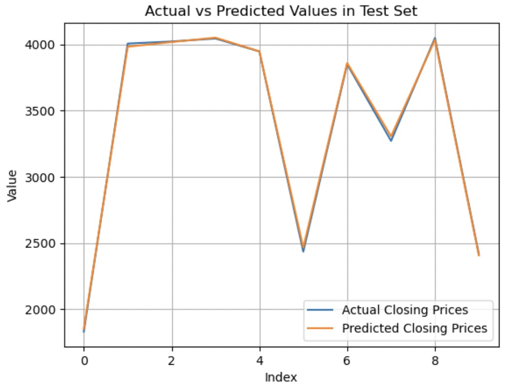
The graph confirms that the model is doing significantly well and can be used for other stock predictions.

Conclusion

So that's how I trained an LSTM deep learning model that can predict stock prices.

Thanks for sticking with me till the end. If you are also interested in making stock predictions, please feel free to use my model and make it even better.

If you think I should change something in the code, you can always drop a comment.

Do like this post if you found it useful.

Catch you in the next one, cheers.

Uday