


pic credit: Unsplash
The Titanic Kaggle Competition is one of the "Getting Started" competitions for data science and machine learning practitioners. It's an open competition and the dataset is quite famous actually. Even ChatGPT knows it.
I trained different machine learning models that can learn from the dataset. This blog showcases the preprocessing steps I used, the models I trained and the performance comparisons between them. Without further ado, let's begin.
About the competition
The objective of the competition is to build a model that can predict if a passenger onboard the Titanic would have survived given some data points about each passenger.
The model would take into consideration data points such as gender, age, ticket class etc. and try to predict if the passenger had a better chance of survival.
Exploring the dataset
As with any machine learning model building, I started with exploratory data analysis (EDA) to get a feel for the dataset. Here's my Kaggle notebook if you wanna follow along.
# read data
train_data_df = pd.read_csv('/kaggle/input/titanic/train.csv')
# check data
train_data_df.head()
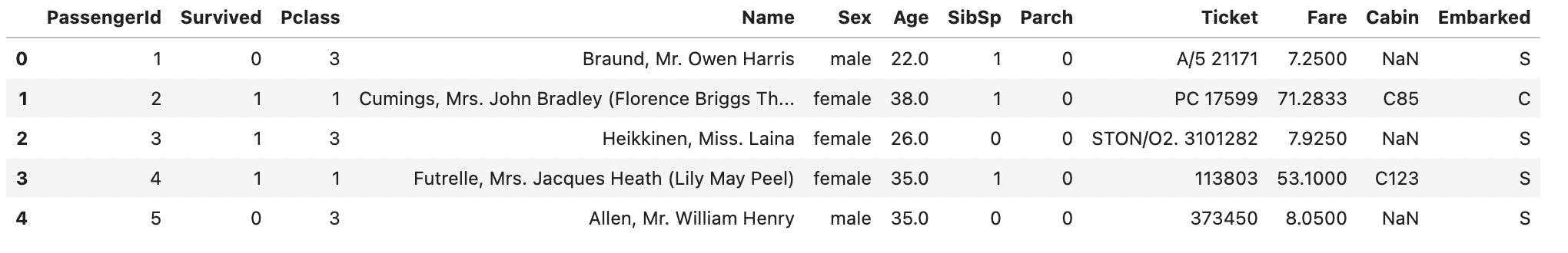
To understand the feature provided in the dataset, we can use the data dictionary provided by Kaggle.
| Variable | Definition | Key |
| survival | Survival | 0 = No, 1 = Yes |
| pclass | Ticket class | 1 = 1st, 2 = 2nd, 3 = 3rd |
| sex | Sex | |
| Age | Age in years | |
| sibsp | # of siblings / spouses aboard the Titanic | |
| parch | # of parents / children aboard the Titanic | |
| ticket | Ticket number | |
| fare | Passenger fare | |
| cabin | Cabin number | |
| embarked | Port of Embarkation | C = Cherbourg, Q = Queenstown, S = Southampton |
# check shape
train_data_df.shape
Output: (891, 12)
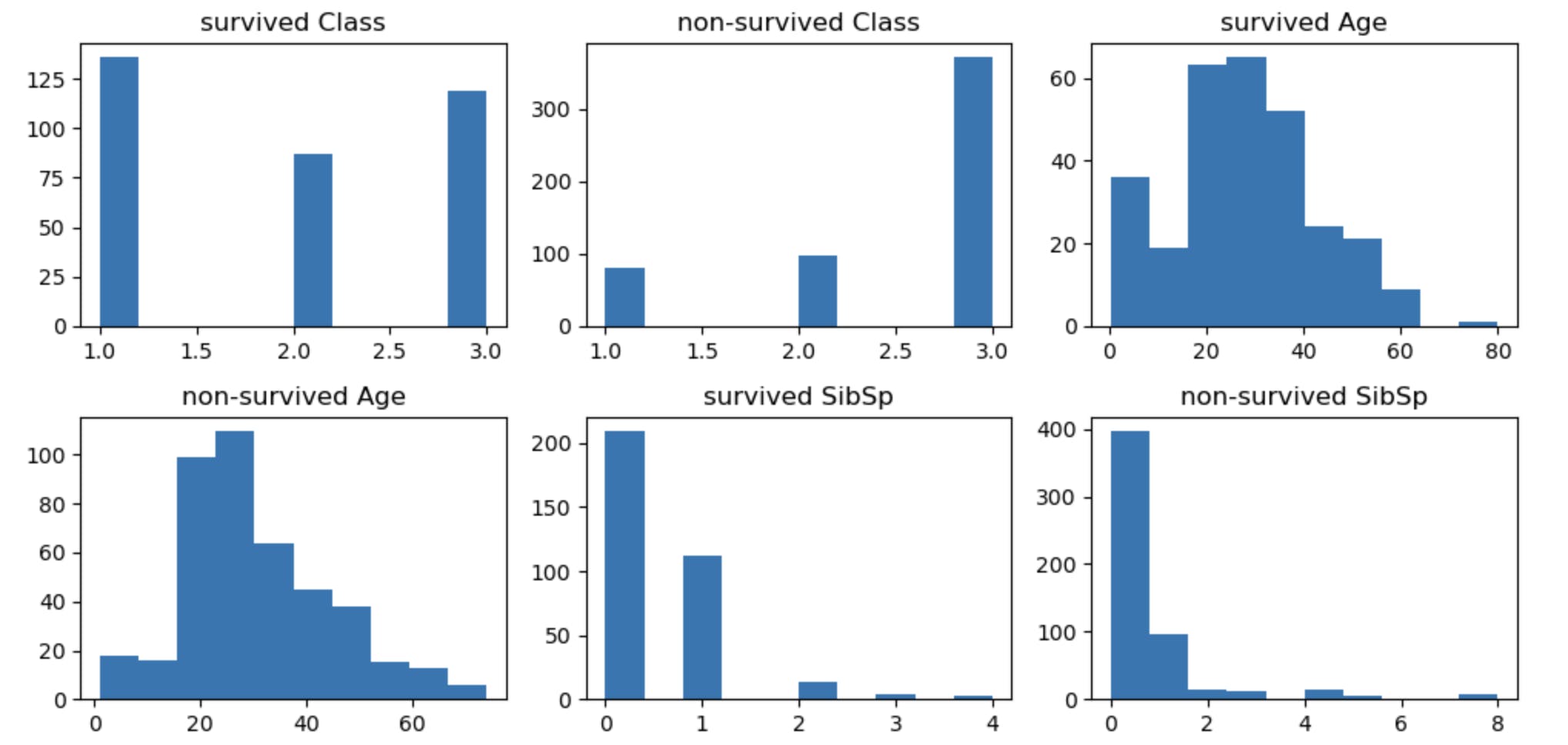
Check relationships among the features
# Create a subplot with 1 row and 2 columns
fig, axes = plt.subplots(nrows=2, ncols=3, figsize=(10, 5))

axes[0][0].hist(train_data_df[train_data_df.Survived == 1]['Pclass'])
axes[0][0].set_title('survived Class')

axes[0][1].hist(train_data_df[train_data_df.Survived != 1]['Pclass'])
axes[0][1].set_title('non-survived Class')

axes[0][2].hist(train_data_df[train_data_df.Survived == 1]['Age'])
axes[0][2].set_title('survived Age')

axes[1][0].hist(train_data_df[train_data_df.Survived != 1]['Age'])
axes[1][0].set_title('non-survived Age')

axes[1][1].hist(train_data_df[train_data_df.Survived == 1]['SibSp'])
axes[1][1].set_title('survived SibSp')

axes[1][2].hist(train_data_df[train_data_df.Survived != 1]['SibSp'])
axes[1][2].set_title('non-survived SibSp')

plt.tight_layout()
plt.show()
Preprocessing
# check for null values
train_data_df.isna().sum()
PassengerId      0
Survived         0
Pclass           0
Name             0
Sex              0
Age            177
SibSp            0
Parch            0
Ticket           0
Fare             0
Cabin          687
Embarked         2
# impute age with median
train_data_df['Age'].fillna(train_data_df['Age'].median(),inplace=True)
# check for null values
train_data_df.isna().sum()
PassengerId      0
Survived         0
Pclass           0
Name             0
Sex              0
Age              0
SibSp            0
Parch            0
Ticket           0
Fare             0
Cabin          687
Embarked         2
dtype: int64
# drop cabin column
train_data_df.drop('Cabin',axis=1,inplace=True)
# drop name column, ticket column
train_data_df.drop(["Name","Ticket"],axis=1,inplace=True)
# drop passenger id
train_data_df.drop(["PassengerId"],axis=1,inplace=True)
# convert age as int
train_data_df['Age'] = train_data_df['Age'].astype(int)
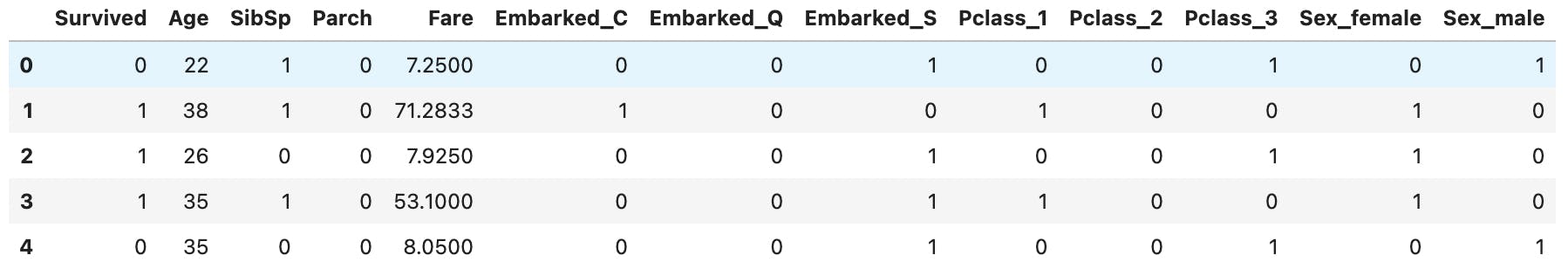
# one hot encode Embarked column and drop it from the original df
encoded_df = pd.get_dummies(train_data_df['Embarked'], prefix='Embarked')
df_encoded = pd.concat([train_data_df, encoded_df], axis=1)
df_encoded = df_encoded.drop('Embarked', axis=1)
# one hot encode Class column and drop it from the original df
encoded_df = pd.get_dummies(df_encoded['Pclass'], prefix='Pclass')
df_encoded = pd.concat([df_encoded, encoded_df], axis=1)
df_encoded = df_encoded.drop('Pclass', axis=1)
# one hot encode Sex column and drop it from the original df
encoded_df = pd.get_dummies(df_encoded['Sex'], prefix='Sex')
df_encoded = pd.concat([df_encoded, encoded_df], axis=1)
df_encoded = df_encoded.drop('Sex', axis=1)
df_encoded.head()
# Splitting the data into features and target variable
X = df_encoded.drop('Survived', axis=1)  # Features
y = df_encoded['Survived']  # Target variable
from sklearn.model_selection import train_test_split

# Split the dataset into training and testing sets
X_train, X_test, y_train, y_test = train_test_split(X, y, test_size=0.2, random_state=42)
# scaling
from sklearn.preprocessing import StandardScaler

scaler = StandardScaler()
X_train = scaler.fit_transform(X_train)
X_test = scaler.transform(X_test)
Below are the different models I trained with their respective accuracy scores. At the end, we have a comparison table.
Logistic Regression
from sklearn.linear_model import LogisticRegression
from sklearn.metrics import accuracy_score


# Create a logistic regression model
# lr_model = LogisticRegression()
lr_model = LogisticRegression(penalty='l2', solver='lbfgs', random_state=42)

# Train the model
lr_model.fit(X_train, y_train)

# Predict on the test set
y_pred = lr_model.predict(X_test)

# Calculate accuracy on the test set
accuracy = accuracy_score(y_test, y_pred)
print("Accuracy:", accuracy)
Accuracy: 0.7988826815642458
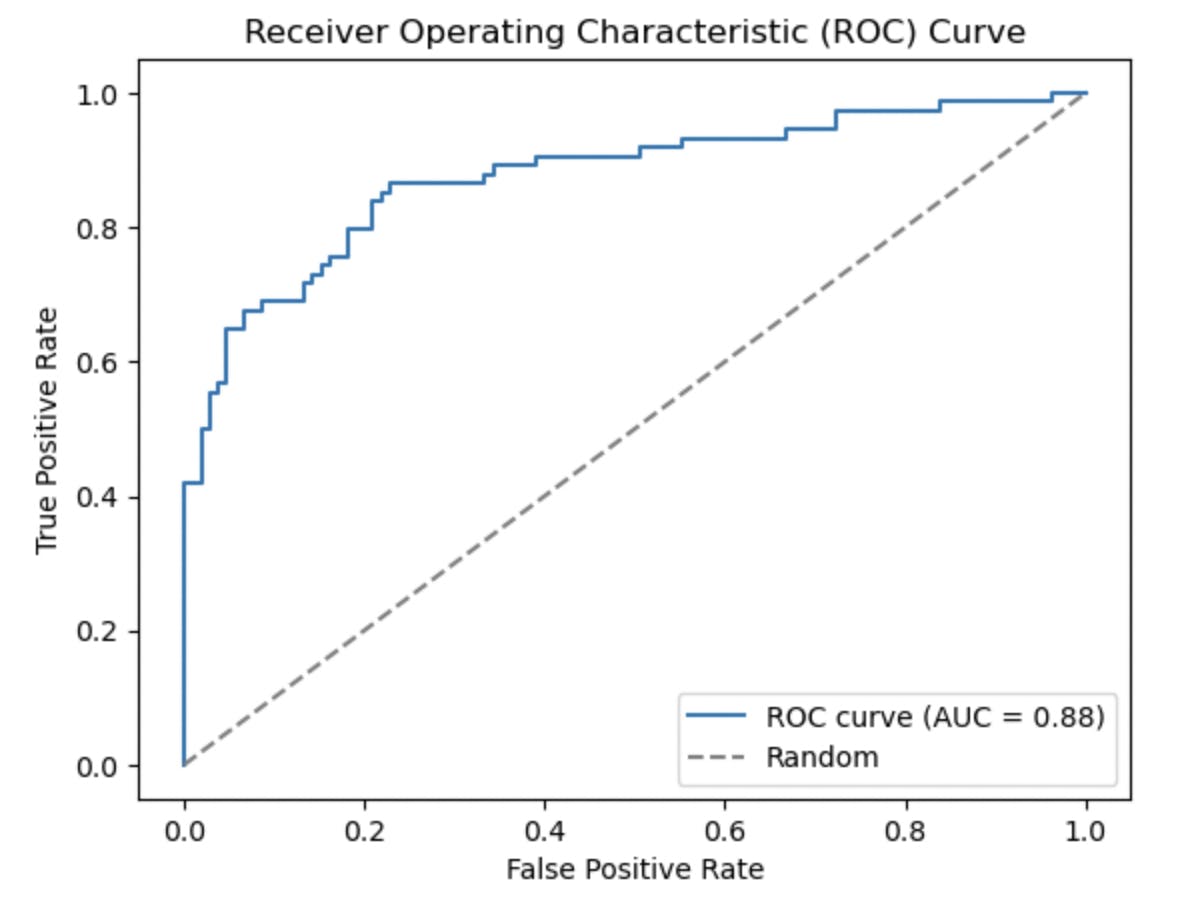
Plotting the ROC Curve
from sklearn.metrics import roc_curve, roc_auc_score
import matplotlib.pyplot as plt

# Predict probabilities for the positive class
y_pred_probs = lr_model.predict_proba(X_test)[:, 1]

# Calculate the ROC curve
fpr, tpr, thresholds = roc_curve(y_test, y_pred_probs)

# Calculate the AUC score
auc_score = roc_auc_score(y_test, y_pred_probs)

# Plot the ROC curve
plt.plot(fpr, tpr, label='ROC curve (AUC = {:.2f})'.format(auc_score))
plt.plot([0, 1], [0, 1], linestyle='--', color='gray', label='Random')
plt.xlabel('False Positive Rate')
plt.ylabel('True Positive Rate')
plt.title('Receiver Operating Characteristic (ROC) Curve')
plt.legend()
plt.show()
Artificial Neural Network
import tensorflow as tf

# Build the ANN model
model = tf.keras.Sequential([
    tf.keras.layers.Dense(32, input_shape=(X_train.shape[1],)),
    tf.keras.layers.BatchNormalization(),  # Add batch normalization layer
    tf.keras.layers.Activation('relu'),  # Apply activation function after batch normalization
    tf.keras.layers.Dense(64),
    tf.keras.layers.BatchNormalization(),
    tf.keras.layers.Activation('relu'),
    tf.keras.layers.Dense(64),
    tf.keras.layers.BatchNormalization(),
    tf.keras.layers.Activation('relu'),
    tf.keras.layers.Dense(128),
    tf.keras.layers.BatchNormalization(),
    tf.keras.layers.Activation('relu'),
    tf.keras.layers.Dense(128),
    tf.keras.layers.BatchNormalization(),
    tf.keras.layers.Activation('relu'),
    tf.keras.layers.Dense(1, activation='sigmoid')
])
# Compile the model
model.compile(optimizer='adam', loss='binary_crossentropy', metrics=['accuracy'])
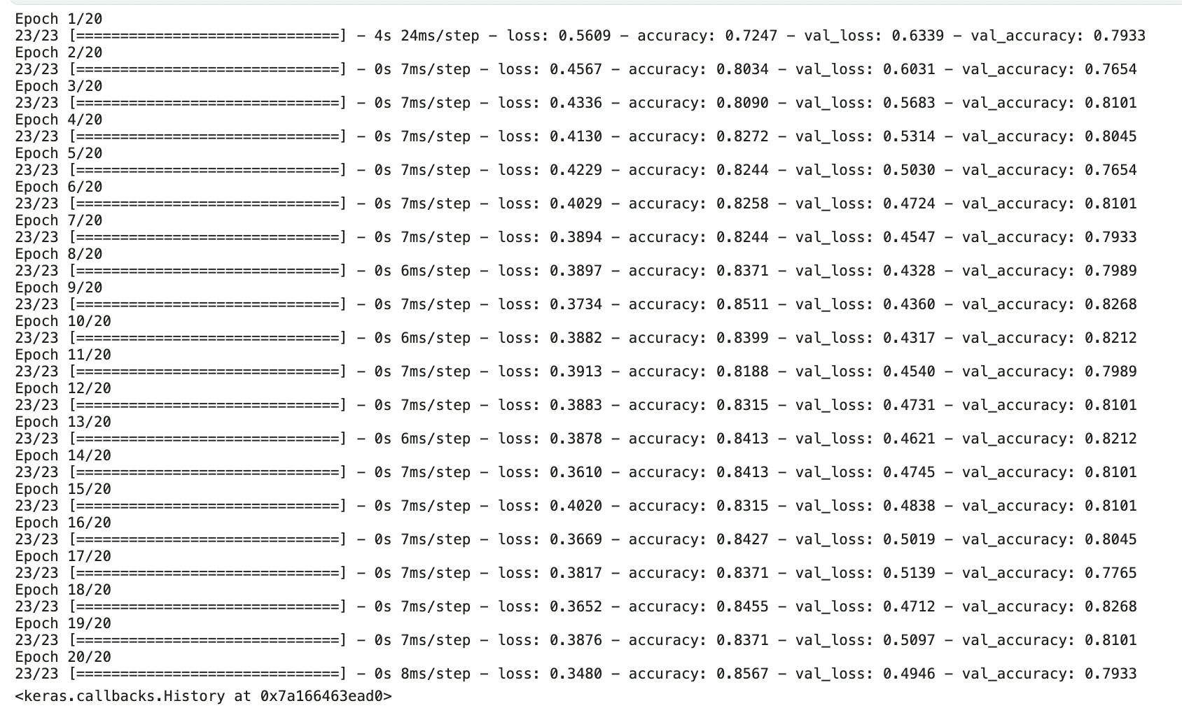
# Train the model
model.fit(X_train, y_train, epochs=20, batch_size=32, validation_data=(X_test, y_test))
Decision Tree Classifier
import pandas as pd
from sklearn.tree import DecisionTreeClassifier
from sklearn.model_selection import train_test_split
from sklearn.metrics import accuracy_score

# Split the dataset into training and testing sets
X_train, X_test, y_train, y_test = train_test_split(X, y, test_size=0.2, random_state=42)

# Create a Decision Tree classifier
dt_classifier = DecisionTreeClassifier(random_state=42)

# Train the classifier
dt_classifier.fit(X_train, y_train)

# Make predictions on the testing set
y_pred = dt_classifier.predict(X_test)

# Evaluate the model
accuracy = accuracy_score(y_test, y_pred)
print(f'Accuracy: {accuracy}')
Accuracy: 0.7821229050279329
Random Forest Classifier with Adaboost
import pandas as pd
from sklearn.ensemble import RandomForestClassifier, AdaBoostClassifier
from sklearn.model_selection import train_test_split
from sklearn.metrics import accuracy_score
from sklearn.preprocessing import OneHotEncoder

# Split the dataset into training and testing sets
X_train, X_test, y_train, y_test = train_test_split(X, y, test_size=0.2, random_state=42)

# Create a Random Forest classifier
rf_classifier = RandomForestClassifier(n_estimators=200, random_state=42)
rf_classifier = AdaBoostClassifier(base_estimator=rf_classifier, n_estimators=100, random_state=42)

# Train the classifier
rf_classifier.fit(X_train, y_train)

# Make predictions on the testing set
y_pred = rf_classifier.predict(X_test)

# Evaluate the model
accuracy = accuracy_score(y_test, y_pred)
print(f'Accuracy: {accuracy}')
Accuracy: 0.8100558659217877
Random Forest with Grid Search
Creating new features from the dataset
# Perform feature engineering and preprocessing
df['Title'] = df['Name'].str.extract(' ([A-Za-z]+)\.')
df['CabinDeck'] = df['Cabin'].str[0]
df['AgeGroup'] = pd.cut(df['Age'], bins=[0, 12, 18, 30, 50, float('inf')], labels=['Child', 'Teenager', 'Young Adult', 'Adult', 'Senior'])
df['FarePerPerson'] = df['Fare'] / (df['SibSp'] + df['Parch'] + 1)
df['TicketPrefix'] = df['Ticket'].str.split().str[0].str.replace(".", "").str.replace("/", "").str.upper()
# Select relevant features and target variable
features = ['Pclass', 'Sex', 'AgeGroup', 'FarePerPerson', 'Embarked', 'Title', 'CabinDeck','TicketPrefix']
target = 'Survived'
X = df[features]
y = df[target]

# Perform train-test split
X_train, X_test, y_train, y_test = train_test_split(X, y, test_size=0.2, random_state=42)

# Perform standard scaling on numeric features
numeric_features = ['Pclass', 'FarePerPerson']
numeric_transformer = StandardScaler()
X_train[numeric_features] = numeric_transformer.fit_transform(X_train[numeric_features])
X_test[numeric_features] = numeric_transformer.transform(X_test[numeric_features])
# Perform one-hot encoding on categorical features
categorical_features = ['Sex', 'AgeGroup', 'Embarked', 'Title', 'CabinDeck', 'TicketPrefix']
categorical_transformer = OneHotEncoder()
# X_train_encoded = pd.get_dummies(X_train, columns=categorical_features, drop_first=True)
# X_test_encoded = pd.get_dummies(X_test, columns=categorical_features, drop_first=True)


# Combine the training and testing data
combined_data = pd.concat([X_train, X_test])

# Apply one-hot encoding on combined data
combined_data_encoded = pd.get_dummies(combined_data, columns=categorical_features, drop_first=True)

# Split the combined data back into training and testing sets
X_train_encoded = combined_data_encoded[:len(X_train)]
X_test_encoded = combined_data_encoded[len(X_train):]
# Define the model
model = RandomForestClassifier()

# Define hyperparameters to tune
parameters = {
    'n_estimators': [100, 200, 300],
    'max_depth': [None, 5, 10],
    'min_samples_split': [2, 5, 10]
}

# Perform grid search to find the best model
grid_search = GridSearchCV(model, parameters, cv=5)
grid_search.fit(X_train_encoded, y_train)
# Evaluate the best model on the test set
best_model = grid_search.best_estimator_
accuracy = best_model.score(X_test_encoded, y_test)
print("Best Model Accuracy:", accuracy)
Best Model Accuracy: 0.8268156424581006
Model Comparison
| MODEL | ACCURACY SCORE |
| logistic regression | 79% |
| artificial neural network | 79% |
| decision tree | 78% |
| random forest with AdaBoost | 81% |
| random forest with new features and GridSearch | 82% |
Conclusion
Overall, I found each of the models to provide similar accuracy. I experimented with several hyper params such as the number of epochs in ANN, increasing the number of trees in random forests etc.
The accuracy scores are pretty decent and this is a good dataset to explore, practice and play around with different machine-learning models.
I hope you found this blog useful. Do leave a like if you did, I'd highly appreciate it.
Cheers,
Uday